What is gradient descent and why should I care?

In each of these cases, we have some quantity that we’re trying to minimise (fuel, carbon footprint, price) whose value depends on a number of inputs whose values can vary. The process of finding the right combination of inputs to give a minimum (or maximum) is called optimization, and it crops up everywhere. 

Optimization problems often depend on many, many inputs, so even though we might be able to  write down a mathematical formula for the quantity we're trying to optimise, finding the optimum value can be very hard to do analytically (i.e. with just pen and paper). As a result, nowadays people mostly try to solve optimization problems computationally. Enter gradient descent, a very popular method for finding minima (and since you can turn a maximum into a minimum by flipping the function upside down (i.e. by multiplying the function by -1), gradient descent also works for maximisation too!) for a wide variety of optimization problems.

The basics of gradient descent

To understand the intuition behind gradient descent, let's look at a very simplified example. Suppose we’re producing lithium-ion batteries for electric cars, and the cost of producing the batteries only depends on how many batteries we produce. This isn’t a completely ridiculous assumption; initially, producing more batteries probably means that we can benefit from increasing bulk discounts for the components, so costs will go down as the number of batteries manufactured increases. But eventually we’ll be producing so many batteries that we’ll need to go to additional more expensive suppliers for our components, so costs will start to rise again. Our goal is to find the number of batteries to produce which gives us the lowest cost.

Our cost function for producing Li batteries might look like this:

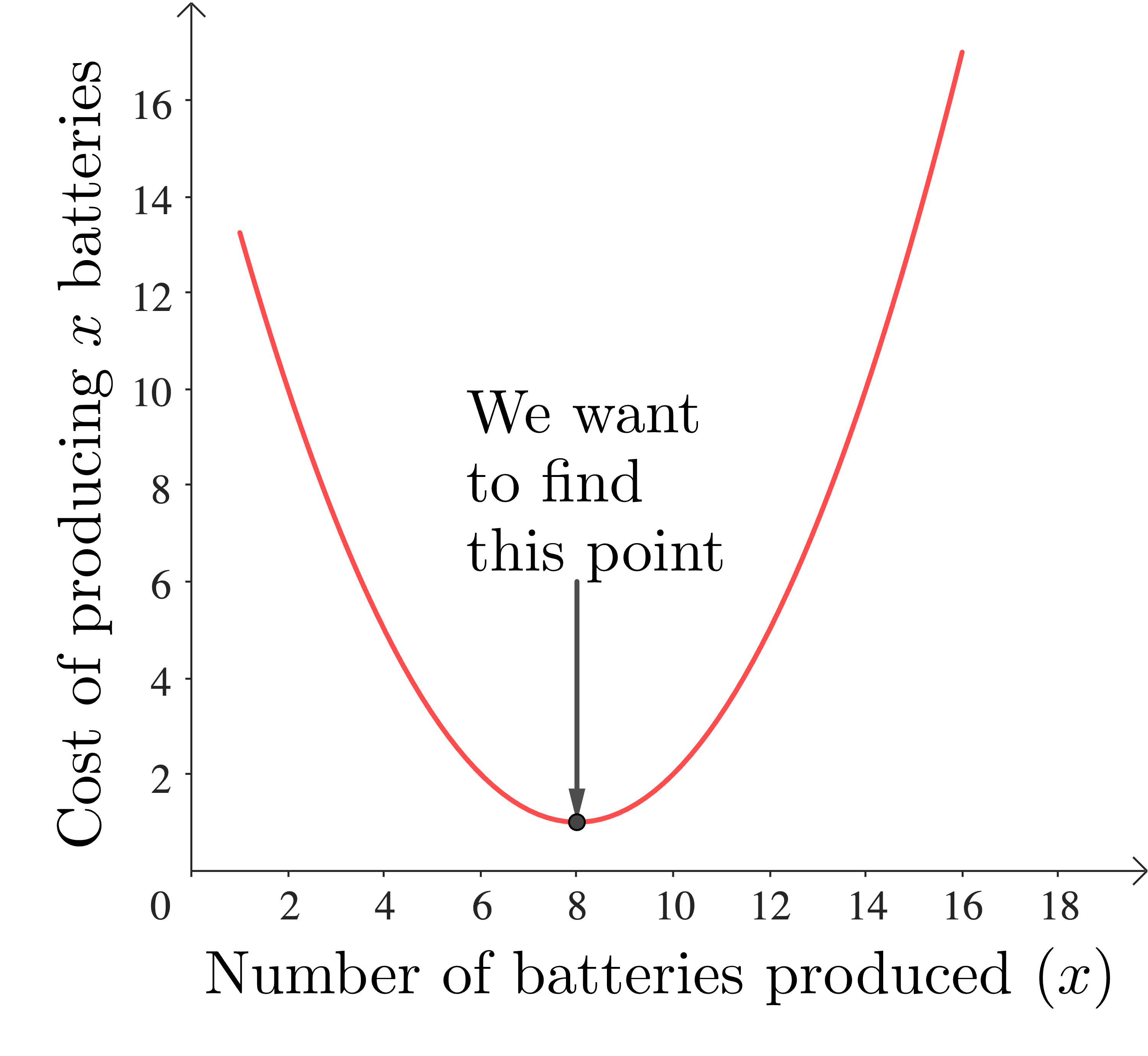
In this example we can just read the answer off the graph (8 batteries gives us the lowest cost), but what we’d like to do is have a method that doesn’t depend on our insight; we want to be able to tell a computer how to find the minimum in a routinized way.

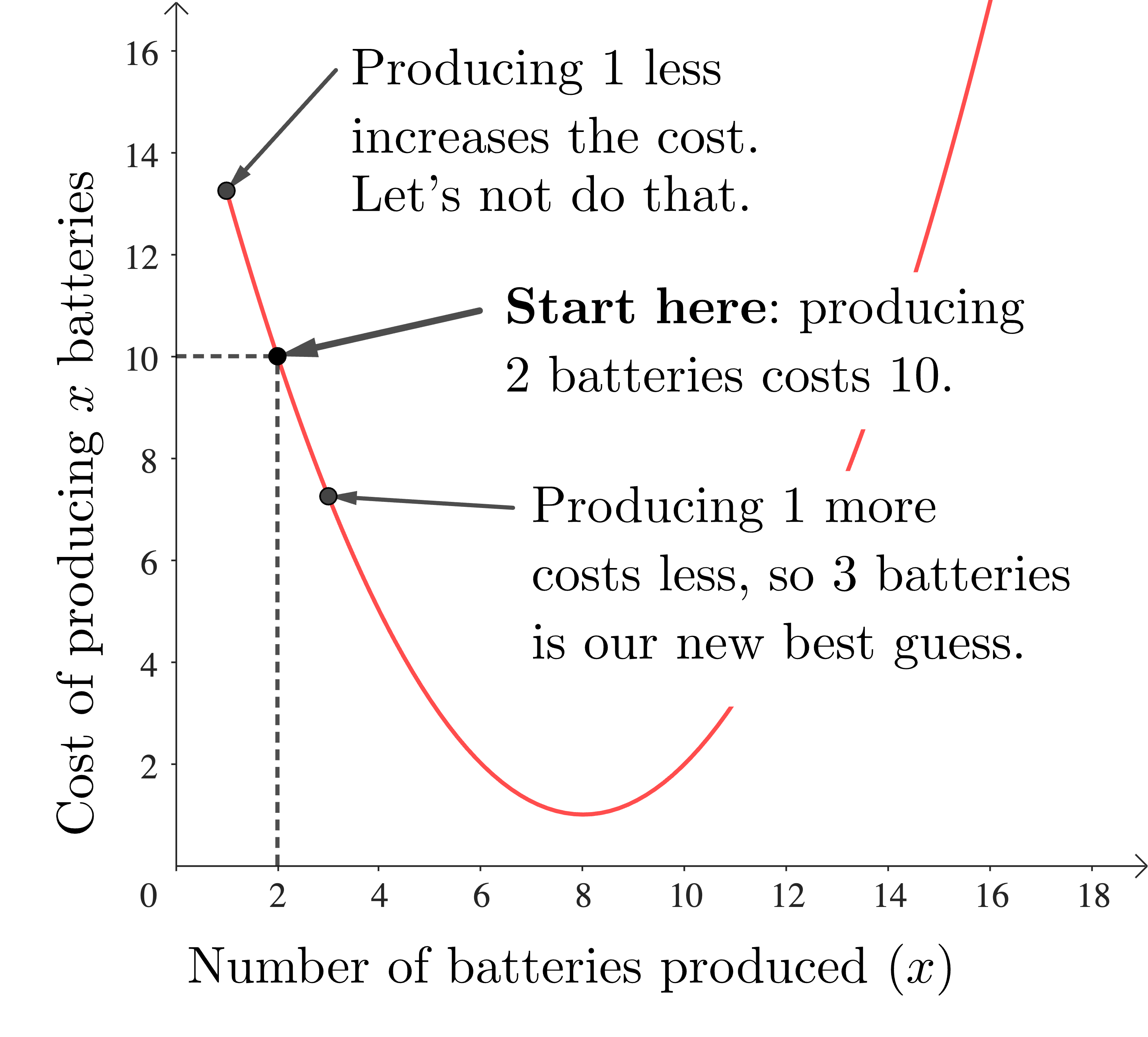
We start by picking some random number of batteries to produce, and finding the corresponding cost. For example, we might pick 2 batteries. Next we look at the cost of producing one more battery, and also one less. We can see that producing 3 batteries is going to give us a lower cost than producing 2, while producing only 1 battery will give us a higher cost than producing 2, so producing 3 batteries is already better than producing 2 batteries. We update our best production level to 3 batteries.

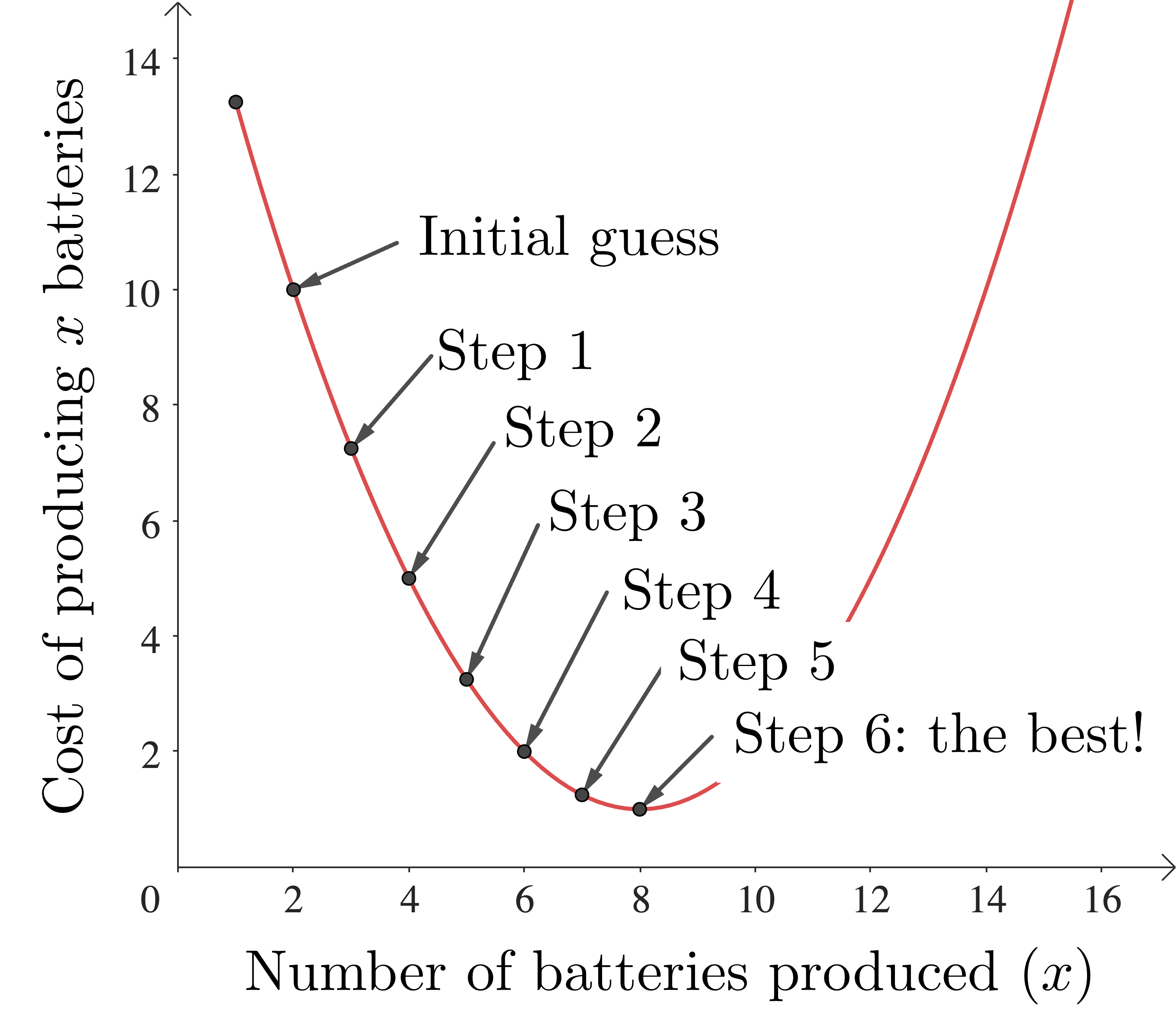
Now we repeat the process, but starting with 3 batteries. Again we see that increasing production, this time to 4 batteries, will lower the cost. If we keep doing this, eventually we will get to a production level of 8 batteries. At this level, increasing or decreasing the production level increases the cost, so we stop - we have found our optimal production level which gives a cost minimum.

This is gradient descent in a nutshell: 

1. start somewhere
2. find the direction in which a small step in the input variable(s) decreases the cost function
3. move a little in this direction and find the cost at this new value of the input variable(s)
4. Repeat from 2. until you get to a point where going in any direction increases the cost.

At that point you are at a minimum. Congratulations!

In practice there are mathematical quantities that we can calculate based on our cost function which will tell us which direction to move in to decrease the cost function most quickly, so we don’t have to check multiple directions in step 2. If you want to know more about them, then there are some details at the end of this article. 

Now gradient descent has been around for a long time (at least since 1847, when Augustin-Louis Cauchy first wrote about it), but using it for optimising complicated functions only really became practical with modern computers, because honestly life is too short to do all these calculations by hand. What has really caused gradient descent to become ubiquitous is the rise of data science, because it is the basis of many of the algorithms used by data scientists in all disciplines.

All of this is of course great (yay, maths in the real world) but there are some problems with gradient descent which our simple example doesn't show, but which crop up in many everyday applications and can make it very slow and computationally expensive. These issues need to be addressed for gradient descent to be used practically.

Gradient descent in practice

Most cost functions are more complicated than our example, and this often means that they have multiple minima. Which minimum gets found by gradient descent depends where we start:

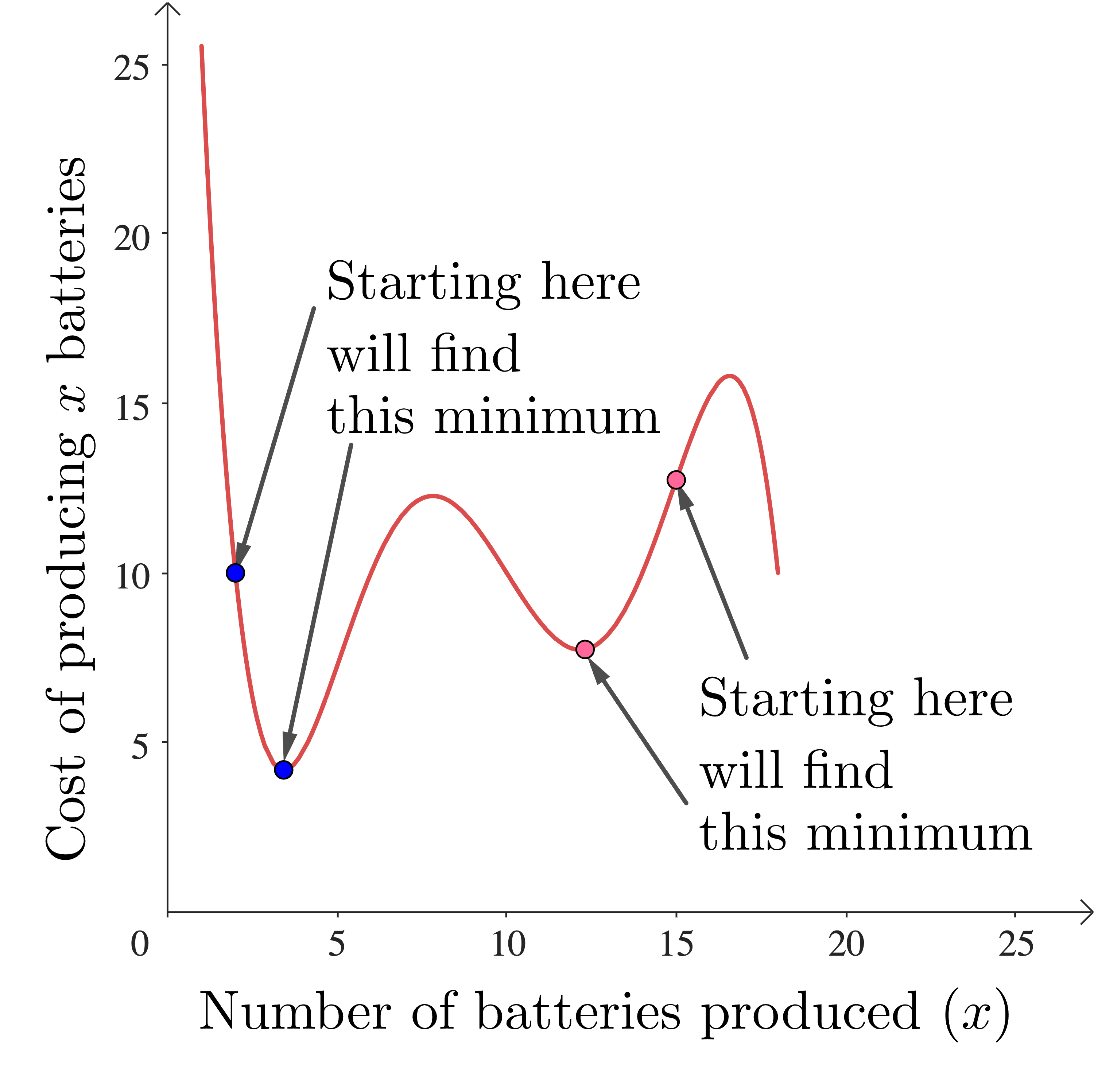
In practice this means that we really need to run our gradient descent from a bunch of different starting points, until we (hopefully) find the “best” minimum. Running the algorithm multiple times for different starting points means that more computing time is used.

The cost functions that arise in today’s applications also have many more than one input - sometimes even thousands. With two inputs, we can visualise the function as a surface:

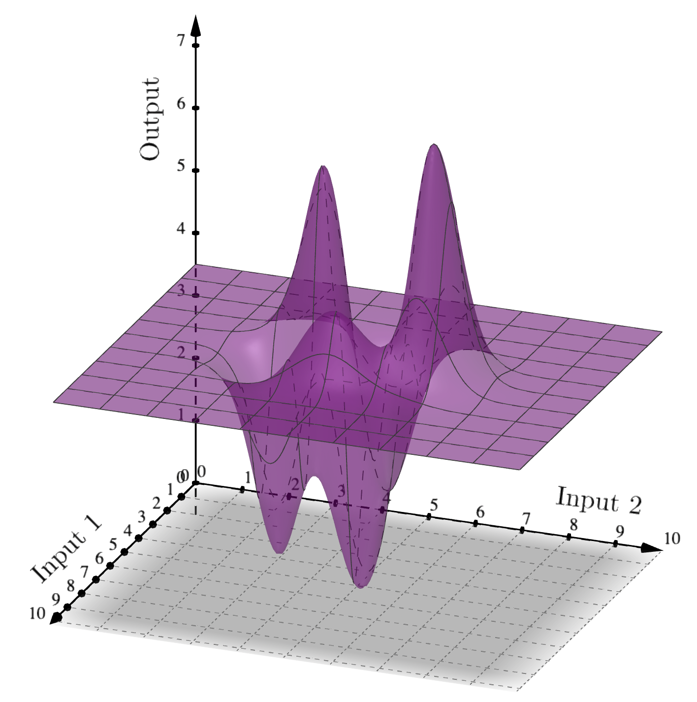
As the number of inputs increases, the space needed for computations increases, and usually the time to perform computations increases too. 

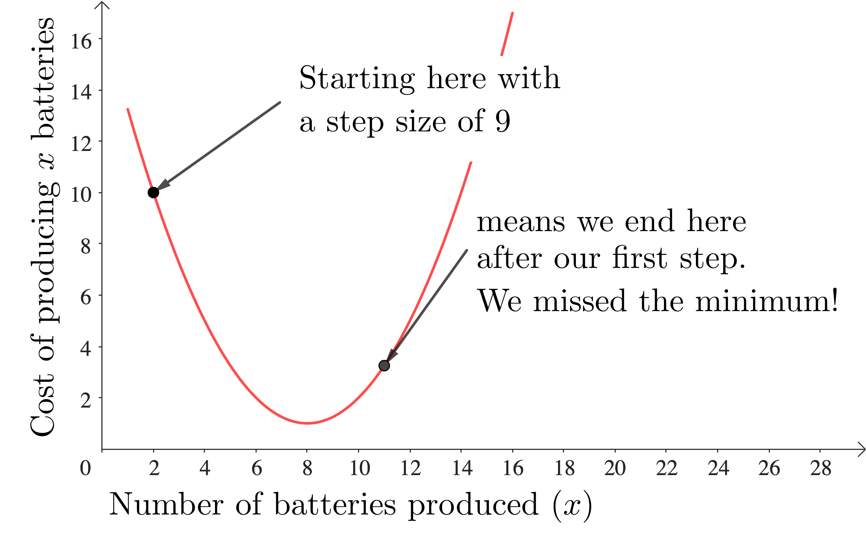
One further consideration in implementing gradient descent is step size. In our simple example we just moved one unit in the input each time we recalculated, but there’s no reason why we couldn’t have taken bigger or smaller steps. Taking smaller steps means that it’s going to take longer to get to any minima, but it does mean that our answer might be more accurate. Taking bigger steps, on the other hand, might mean reaching the minimum quicker, but it could also result in missing the minimum entirely!

Picking the step size that is optimal for a particular problem requires some thought. There’s no reason why the step size has to be the same for each iteration, for example, and there are many methods for adapting the step size optimally.

Putting these issues together results in a situation where the basic gradient descent which we first discussed can take a lot of computational time and space. As a result, there’s been a lot of research into improving various aspects of gradient descent. For example, Yurii Nesterov developed an improved version of gradient descent that can quite drastically speed up the computation time for a large class of optimization problems called convex problems. You'll be able to read more about convex optimization in the next article!

Going a bit deeper

As I mentioned, there are mathematical quantities that we can calculate based on our cost function which will tell us which direction to move to decrease the cost function most quickly. For cost functions of one variable, like our simple example, the derivative tells us which direction to move in to decrease the cost function. You can learn about this in a first course on calculus (e.g. Kahn Academy)

For cost functions of more than one variable we need a related concept, the gradient, which crops up in multivariate calculus. The gradient tells us which direction to go in order to increase the function as fast as possible, so going in the opposite direction will decrease the function as fast as possible. Hence the name “gradient descent”. If you’ve done a little calculus, then mathinsight.org gives a great mathematical introduction to the gradient. 3blue1brown has a fabulous introduction (with animations) to gradient descent for neural networks, which doesn’t require extensive understanding of the gradient.

For a deeper dive into the maths behind gradient descent (and everything else you need for data science) I highly recommend Andrew Ng’s course Mathematics for Machine Learning and Data Science.

If you’d like to read more about Yurii Nesterov and his work, then we have an interview with him here.

Written by Dr. Claire Blackman.