Getting to optimal: why convexity matters

If you read the recent NCCR Automation interview with Yurii Nesterov, or you’ve been learning about optimization, automation or any hot topic in data science, you’ve probably come across the term “convex optimization”. You might even have heard that it plays an important part in new, automation-driven technologies, such as self-driving cars. We touched on the topic in our recent post on gradient descent, but if you want to dig deeper into why it’s so important, read on.
Before we can get to the convex bit, let’s recap what optimization in general is all about. As described in my previous article, mathematical optimization is the process of finding the set of inputs which results in a minimum (or maximum) value for a cost function that depends on these inputs. (You might find it helpful to read, or re-read, that piece before digging in further.)
Sometimes we’re free to choose any combination of inputs, in which case the optimization is said to be unconstrained. Usually, however, we’re limited in how much of an input is available, or what combinations of inputs we can use, to find our optimum – grocery shopping on a budget sadly means no unlimited chocolate. In this case of “constrained optimization”, the set of allowed inputs is called the feasible set.
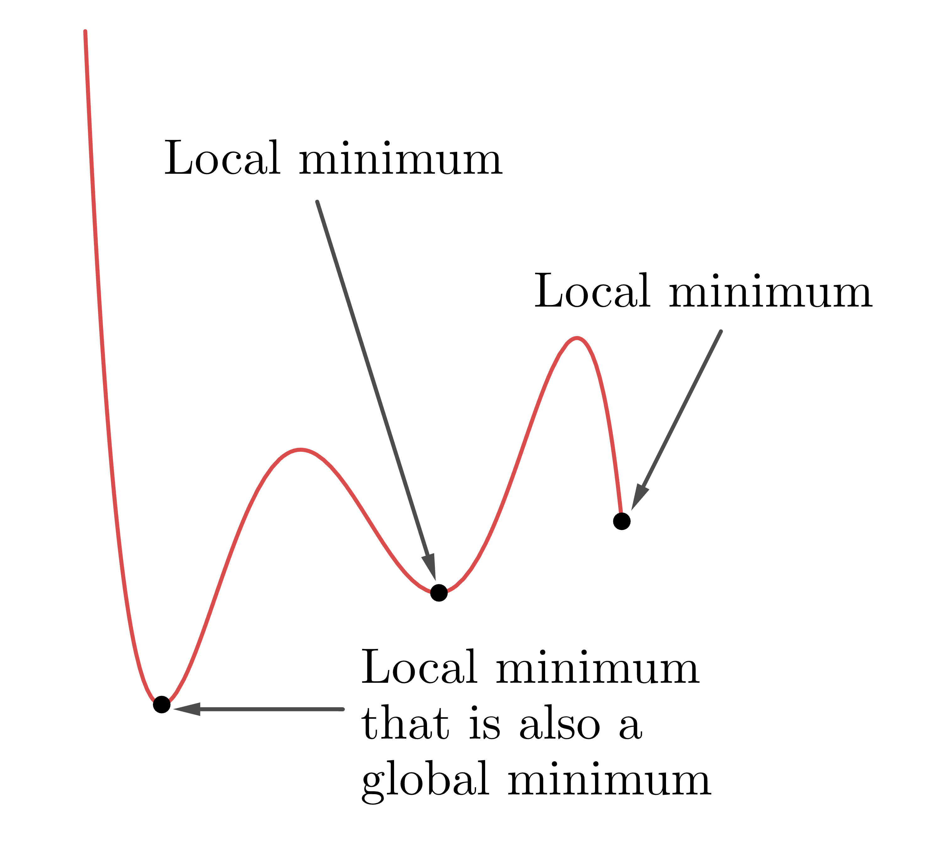
As we’ve seen in gradient descent, some cost functions have multiple minima – the curve dips up and down. Each of these is called a local minimum (because relative to its neighbours, it’s the lowest point), but often what we’re interested in is the lowest of the low: a global minimum. For a function of one variable, local and global minima look like this:
As Yurii Nesterov pointed out in his interview, gradient descent can (usually) find a local minimum, but it can’t tell us how many other minima there are, or if they’re “better”. But often it really matters that we find the global minimum fast, reliably, and to a very good degree of accuracy. More and more we see computers embedded in devices that use optimization to make time-critical choices based on physical data (think self-driving cars). What is key here is that the computer is making real-time decisions with little or no human input – so using an accurate, reliable and efficient optimization method is absolutely crucial.
To find a global minimum, we often need to know more about the shape of the cost function, and this is where the whole convexity thing comes in. We’re actually going to talk about two kinds of convexity, but don’t panic: they’re related, and are pretty straight-forward, sensible ideas!
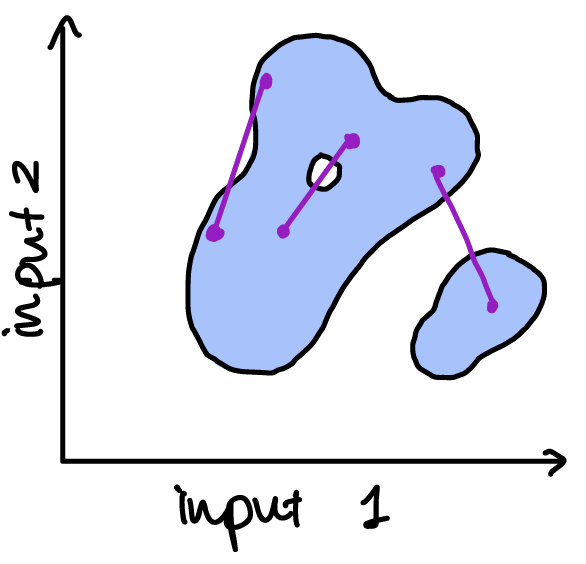
The first type of convexity we need relates to the inputs – it is used to control the shape of the feasible set for our cost function. A set is convex if, whenever we join two points in the set with a line, all the points on the line are also in the set. Pictures will help!
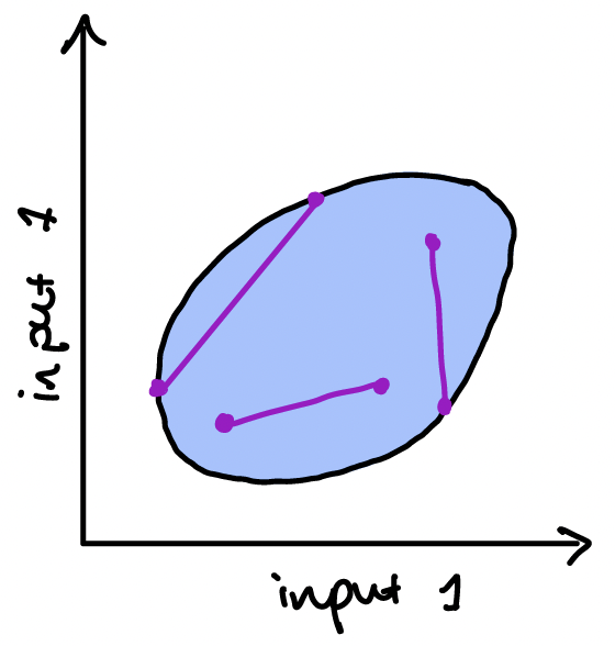
If our input set is one-dimensional, then requiring it to be convex just means that we want it to be a continuous interval.
The second type of convexity tells us about the shape of functions. A function is convex if
- its input set is convex, and
- you can pick any two points on the function, connect them with a straight line segment, and every point of the function between the two points lies on or below this line. If every point of the function between the points lies strictly below the line then the function is called strictly convex.
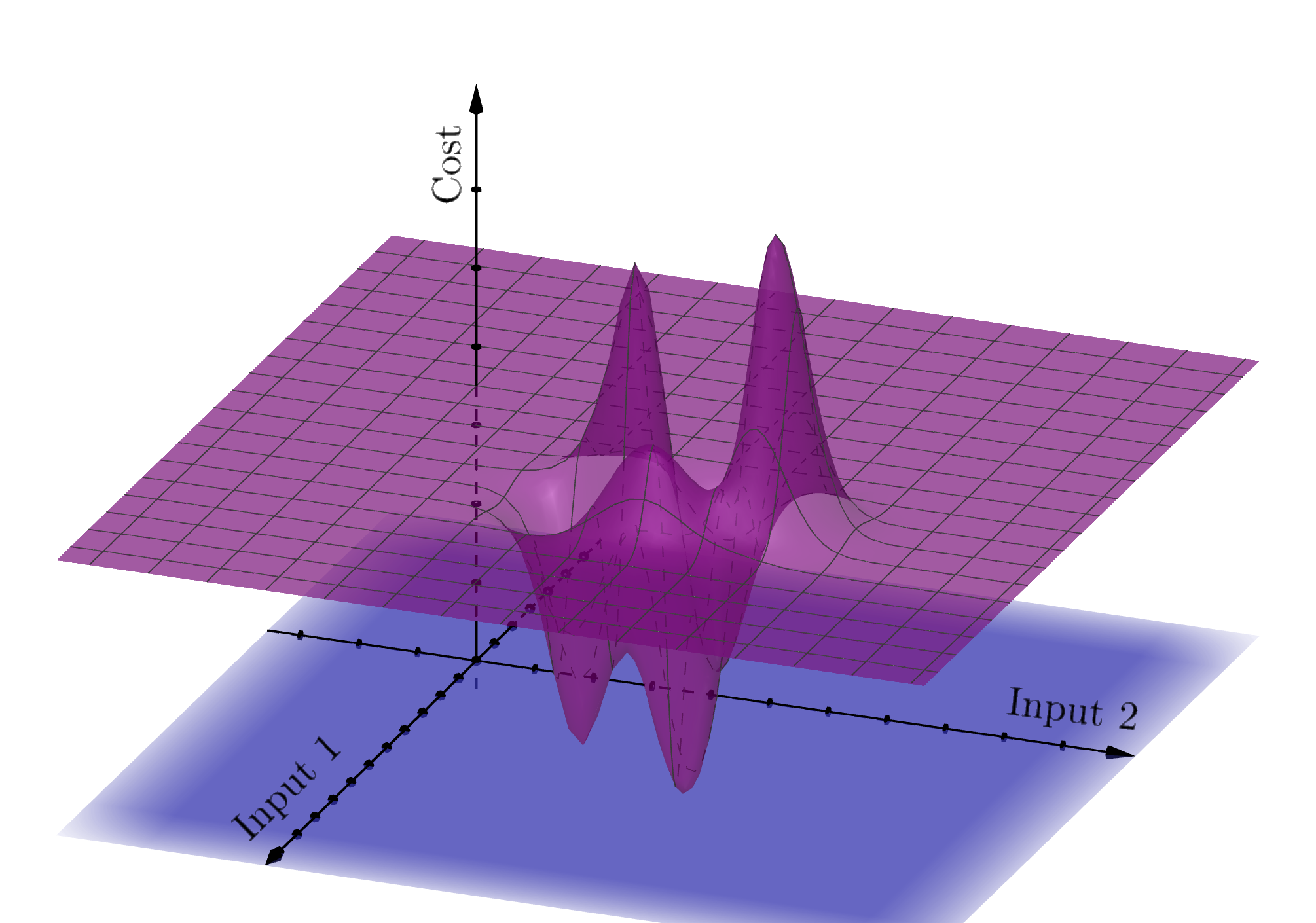
The convexity of the input set isn’t obvious in the previous examples, but it is required to avoid situations like the following, which we’ll see a bit later will give problems:
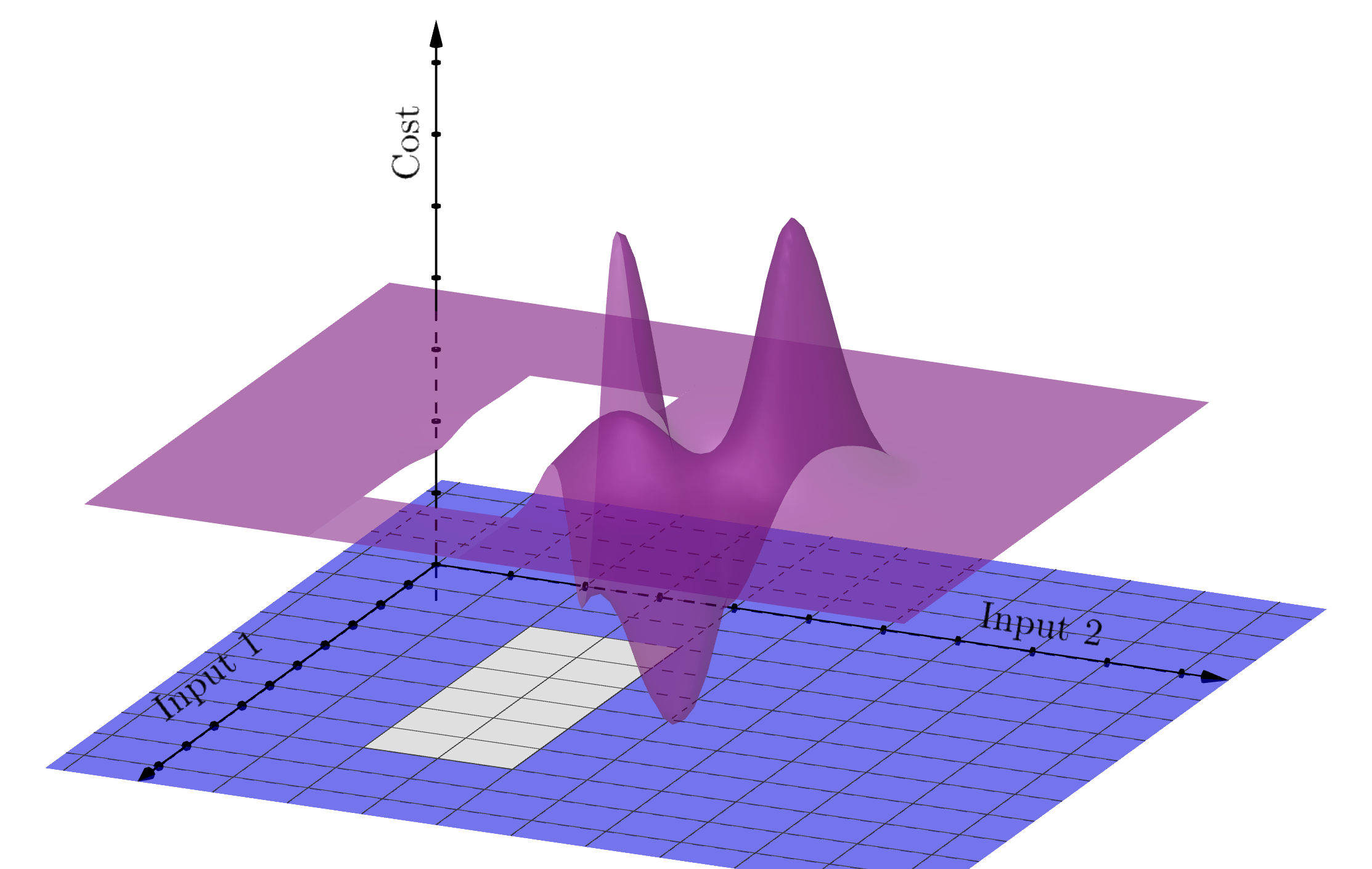
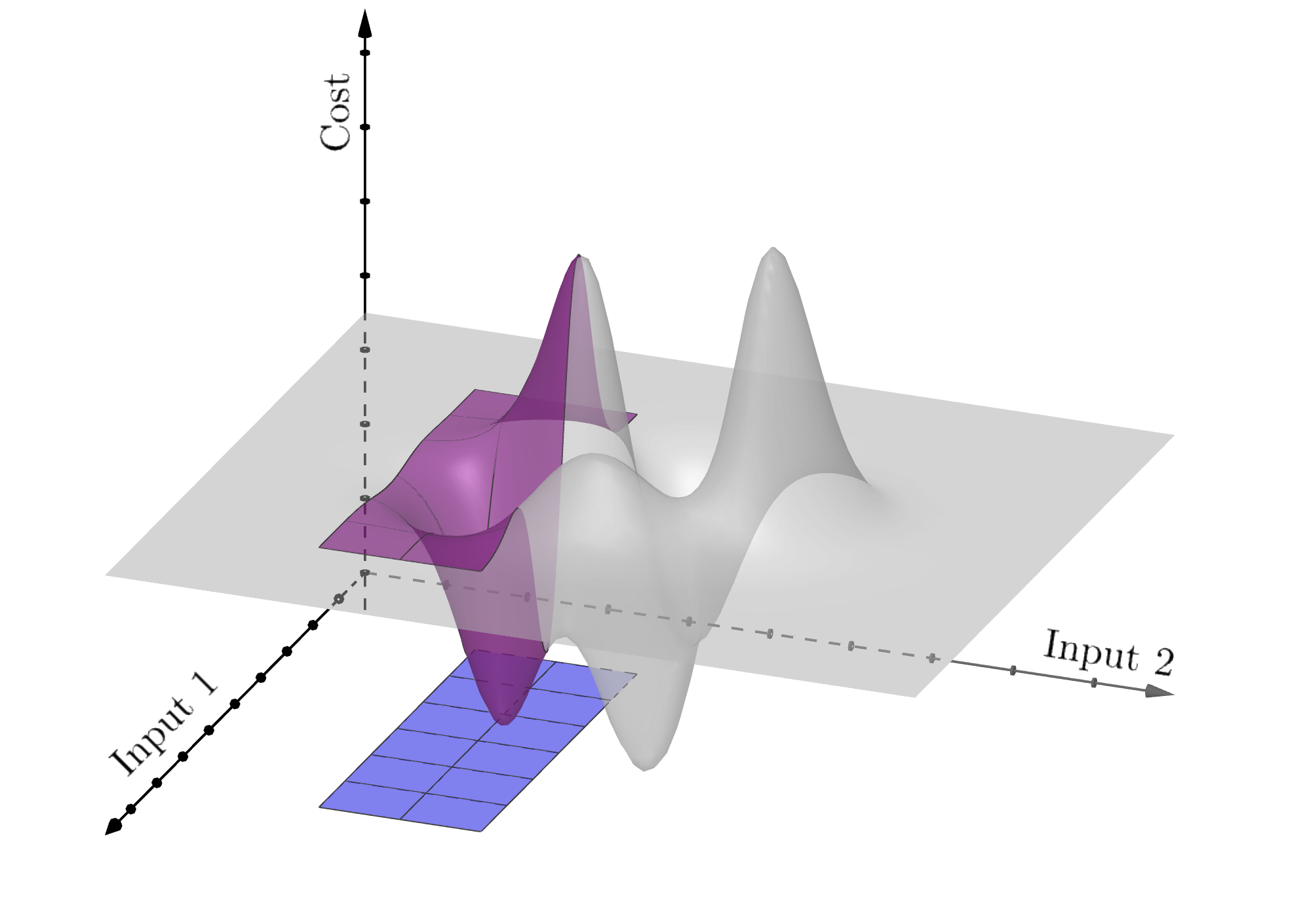
Oh no! In these two examples, the fact that the input set (in blue) isn’t convex results in gaps in the cost function – the function is non-convex because it is discontinuous.
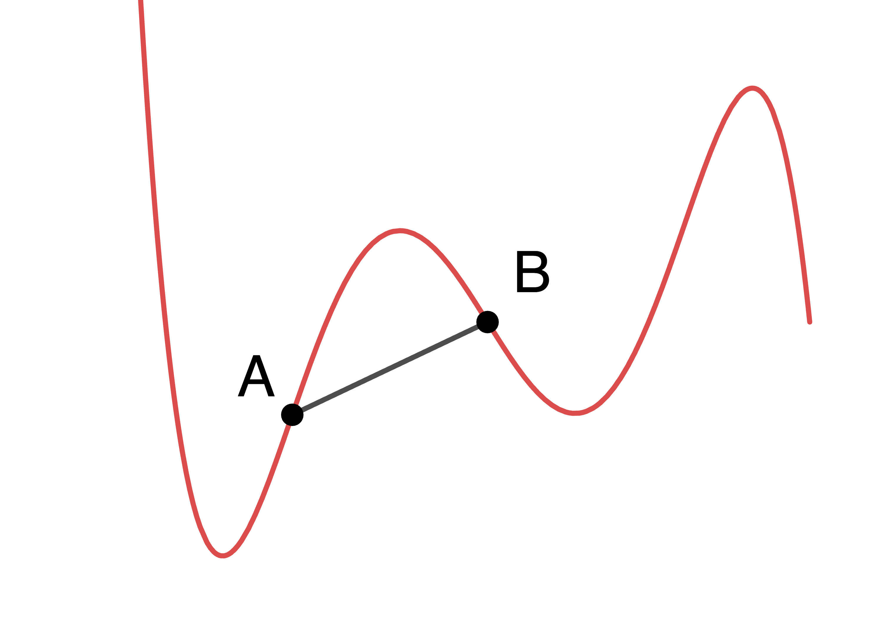
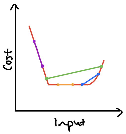
This also shows a non-convex function. Although it has convex regions, if there are any pairs of points for which the joining line lies below the function (instead of the other way around), then the function is non-convex.
To see just how much convexity guarantees about a function’s local and global structure, grab a pen and paper and sketch the following:
A. A convex function with different minima at two different input values
B. A convex function with any minima at two different input values
C. A strictly convex function with minima at two different input values
D. Convex and strictly convex functions with no minima
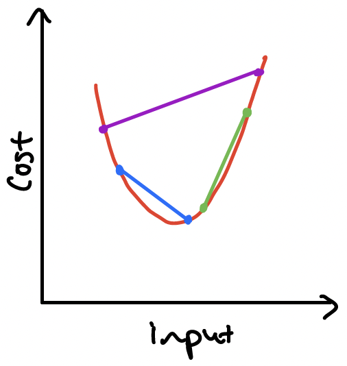
Here’s one way to go about tackling a. and b.:
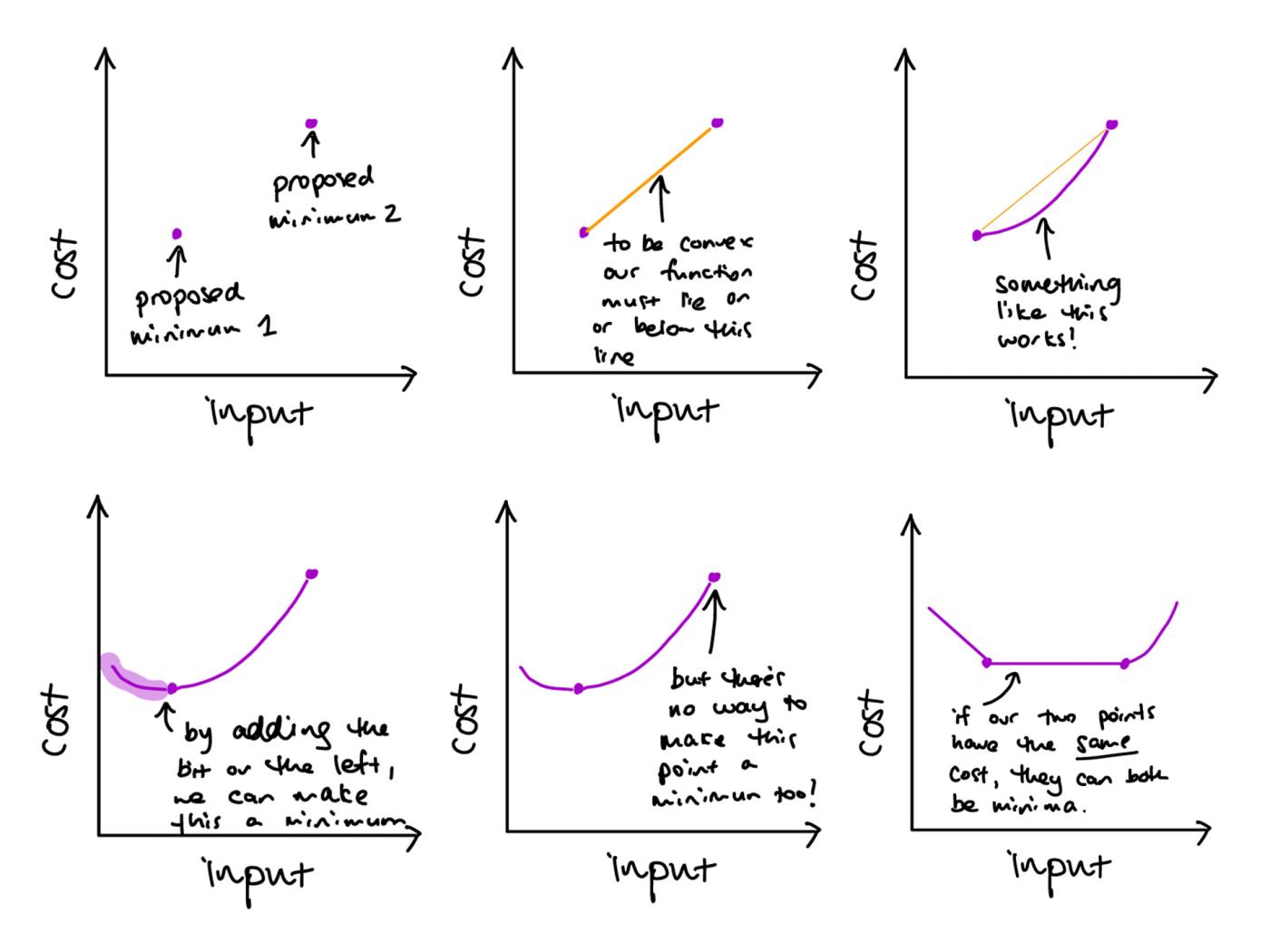
This exercise is a kind of reverse engineering – we’re just looking at what convexity really means. In practice, we would normally be starting with a function and looking to determine the minimum; here, we start with possible cost values and look to see what functions might show them as minima. That helps to demonstrate why convexity matters. From the sketches above we can see that it’s not possible to have a convex function with two minima with different costs, but two minima with the same cost is possible (in which case we’ll probably get a whole lot of other minima too, at all the points between our chosen minima!).
But this isn’t an option for a strictly convex function, because then between our two chosen minima the function would have to be strictly below the joining line – which would mean the original points would not be minima!
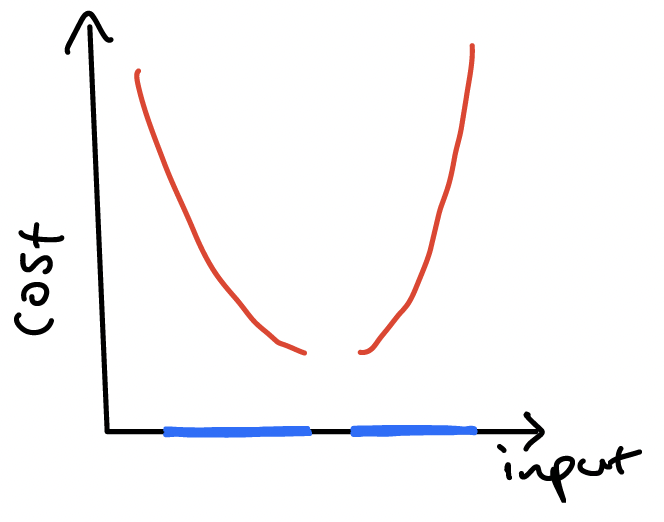
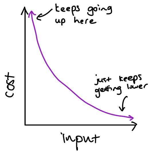
We can however have convex functions without any minima1, like this one:
This leads us to the following important conclusions:
- If our function is convex, then any local minimum is a global minimum (because all minima must have the same cost).
- If our function is strictly convex, then we can say more: there is at most one global minimum. Note that we’re not saying that there definitely is a minimum (we just sketched a convex function with no minimum) – but if there is one, we know it’s the unique global minimum.
This is powerful stuff! Now, if we use gradient descent on a convex function and we find a minimum, we know that it’s the best one. And there’s more. Because convexity tells us so much about how the function changes as we change the inputs, it’s possible to develop cunning algorithms that are fast (e.g. Nesterov’s accelerated gradient descent or interior point methods), extremely accurate and very reliable. As a result, convex optimization – optimization in which the cost function and constraints are convex functions – has seen a huge amount of research since the 1940s, and a growing number of applications since the 1980s.
Convex optimization can also help with non-convex problems! For example, we can use a convex approximation of a non-convex function to find a good starting point for gradient descent, or to find a lower bound for the minimum.
Of course, there is a catch: expressing a problem as a convex optimization problem isn’t always straightforward. With non-convex functions, it’s usually pretty clear how to write down the cost function and constraints, but as we’ve seen, finding minima is more art than science. With convex functions, the situation is reversed: writing the problem so that the functions involved are convex is more of an art than a science (although there are helpful techniques to try), but once the problem is written down, there are efficient, accurate, robust methods for finding the minimum. And that is the magic key that unlocks so much possibility in automation.
1 For extra credit: does this remain true if we limit the input set?
Written by Dr. Claire Blackman.