What is MPC anyway?


Driverless cars, which 50 years ago seemed to be a futuristic dream, are driving on our roads and creating headlines in our news feeds. In the area of railway transport, a quieter revolution is taking place. Since trains move along fixed tracks, and don’t have the whole issue of dealing with other vehicles or pedestrians getting in the way (hopefully), the problem of automation might seem much simpler to solve, and indeed, there are already quite a few driverless train systems in operation. Most of these are passenger metro systems, although the world's longest driverless train system is the Rio Tinto Iron Ore system in Western Australia, with a longest train journey of over 500kms. With the current increased focus on energy efficiency, the question around driverless train systems has shifted from “How do we do it?” to “How do we do it right?”.
To understand how this question can be answered using Model Predictive Control, we’ll start at the beginning.
The factors which determine how fast a train is moving at a given point on the track are:
- The electrical force applied to the train. This is a positive force if the train is accelerating, and a negative force if the train is braking. Regenerative braking slows the train by using the motors as generators and sending the recovered energy back to the grid.
- The pneumatic breaking force (produced by traditional breaking using friction). For most modern trains, this is only used in emergency situations.
- The forces due to the slope and curvature of the track
- The rolling resistance force
- The mass of the train
Of these, we can only control the electrical and pneumatic forces that are applied. We can, however, model the rest of the forces (more about this later), enabling us to calculate the electrical forces needed to move the train at a particular speed. But what speed should that be? This will be determined by the additional criteria which need to be taken into account:
- The total energy drawn from the grid should be minimised
- The laws of physics shouldn’t be broken
- Speed limits should be adhered to
- Travel times should be adhered to
- The physical limitations of the train controls shouldn’t be violated
- The maximum possible power to the wheels shouldn’t be exceeded
The forces and criteria combine to give a set of equations which need to be solved together to find the optimal electrical force over the trip. In simple cases it’s possible to find a continuous electrical force which satisfies the forces and criteria; the required electrical force for an idealised two-dimensional train trip up a hill might look something like this:
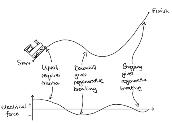
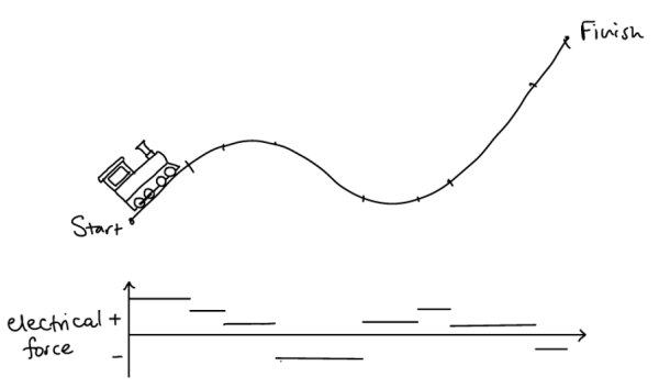
Unfortunately, traditional analytical methods that give a continuous function for the electrical force have drawbacks: they rely on simplifying assumptions that don’t hold in practice and require expert knowledge to adapt the solution algorithm if the problem formulation changes . One way to overcome these issues is to use numerical methods. In these methods, we first discretise the problem by splitting the track up into sections which each have a constant slope and speed limit. We then find a solution which has a constant electrical force on each section.
This solution would work very well if:
- The model of the system was perfect. This means knowing exactly how much the train weighs, for example.
- There are no disturbances, such as wind, or rain changing the track conditions.
Unfortunately, of course, these things can’t generally be known accurately enough or predicted. Since the acceleration of the train depends on the mass of the train, if the mass is not known accurately enough (e.g. by not knowing how many passengers are inside) the acceleration might be too high (resulting in the train breaking the speed limit and using too much energy) or too low (resulting in the journey taking too long).
This is where Model Predictive Control can help. Here’s how it works: before the train starts, the optimal electrical force for the trip is calculated, based on the best available information. However, this calculated electrical force is only used at the start of the trip. After a small amount of time has elapsed, sensors gather information about the current position, speed and acceleration of the train. Based on this information, a new optimal trip is calculated for the remaining part of the track, and a revised force applied. This process of getting real-time information, recalculating the optimal trip and updating the applied force is repeated regularly throughout the trip, enabling the journey to be adapted and optimised on the fly:
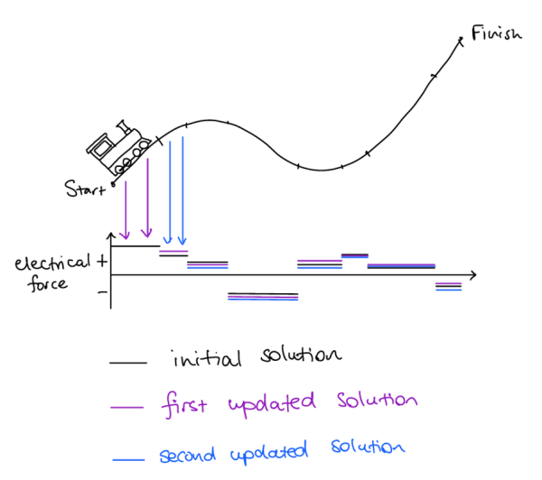
This is a potentially extremely powerful technique, as not only can the energy usage be minimised, but unexpected timetable requirements or temporary speed restrictions can be seamlessly integrated into the trip plan.
In the NCCR Automation-funded project SWITONIC, Dimitris and Juxhino have been evaluating its potential in the real world. They deployed the algorithm on a modern electric train and benchmarked it against popular industry solutions on a 20 km track. Encouraged by the results, they decided to found nuorail to move this approach from proof-of-concept to production.
Text by Claire Blackman