Via Automation - a small tour of automatic control: Feedback


At first, it might appear strange to discuss automatic control during a hike. Aren’t most of us enjoying hikes precisely to get into nature and away from industrialisation? As we already saw in the previous post, our tools are very much intertwined with effective preservation strategies for our environment, but perhaps more importantly and more directly, viewing controls and optimization as being solely concerned with industry removes many of the fun and useful things that we get up to.
At the end of the day, someone in automatic control aims to understand dynamical systems and how they function on a basic level. These systems could be industrial, but they need not be. We aim to understand in particular how to change dynamical behaviour (ie the patterns of behaviour taking place within a system over time), for instance, to improve accuracy of a 3D printer, to smoothly stabilise airplanes when turning, to efficiently heat coffee machines and even to understand calcium regulation within cows. Believe it or not, all the aforementioned examples (even including the cows) can be studied using more or less the exact same tools and the overarching theme here is feedback.

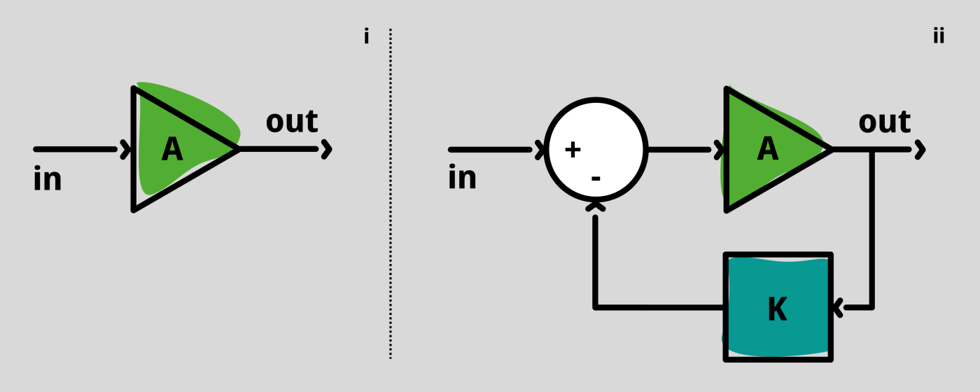
During the early 1900s, the concept of feedback came about in telecommunication. More precisely, over long distances, signals became so weak that information was lost, meaning that engineers had to find a way to amplify them. Schematically and simplified, if we have some input;(in), the output (out) would be out = A*in, see Fig. 1(i). Thus, we need to make sure that amplification (A) is large enough. However, amplifiers at the time were not that reliable, so it was not possible to set a fixed value for A that would always be sufficient. It is as if you were trying to drive while your gas pedal was only working sometimes.
To solve this, Harold Black, an engineer at Bell Labs, came up with feedback. Negative feedback to be precise. For a schematic depiction, see Fig. 1(ii). In this case the output follows the equation out=A/(1+A*K) *in. Hence, if Ais large enough, regardless of being reliable or not, we get that out is roughly equal to 1/K*in.
Note, in this case you may think of ‘inʼ more as a ‘reference signalʼ. These schematics were implemented using analogue components and the beauty is that, although amplifiers are active elements and hence can be unreliable, the feedback gain would always be reliable as it can be implemented using passive components. This observation turned out to be revolutionary.
You can read more about this discovery in the marvellous book by Gertner [2]. As you will note, Bell Labs was in general far ahead of its time (a Picturephone?). It is also interesting to see how institutions like Bell Labs inspired research institutions nowadays [ch. 20, 2]. For more historical and technical remarks you might also want to listen to Ep. 38 of the inControl podcast [3].
The schematic above is arguably the simplest manifestation of feedback, normally the system is not a constant like A, but a dynamical system where each of the parameters is constantly changing (think of a motor, robot and so forth). However, the example captures the core of this post, in some form, we feed back an error into the system towards obtaining a desirable output.
Letʼs generalise the above and move to a slightly more involved example. Typically, to design feedback schemes, we consider some error that we would like to be 0, say ‘err = in-outʼ, meaning that we want no errors in our system. If, after appropriate scaling we feed this back into the system, then we would call this ‘proportionalʼ (P) control. Our control signal is proportional to the error signal. Now suppose that also a constant, but unknown, disturbance enters the system. Then, in general, to make sure that our error is again 0, our control signal must include a constant term as well, to compensate for the disturbance. However, in that case, the control signal cannot be a function of just the error, for otherwise the error would never go to 0. To reconcile this, the control signal is chosen to be proportional to the ;integral of the error signal. By appropriate design, the integral of the error will eventually match the disturbance, while the error itself vanishes with increasing time. This is the core of the most important and widely used feedback scheme called ‘PID controlʼ, as introduced in 1922 by Minorsky (1). For the technical readers, you may consider not only the error itself (P) or the integral (I), but also its derivative (D).

This detour brings us back to the herd of cows. Many of you (not me), think of milk when thinking of cows; and part of the biology that underlies the production of milk has a strong link to the feedback concepts just discussed. Specifically, calcium levels within cows are tightly regulated thanks to hormones that seem to use the biological version of a PI controller (4). Around birthing, milk production requires the mother cow to provide calcium, which causes her levels to drop to a dangerously low level, and a hormonal feedback mechanism is activated.
If this looks familiar, it’s because it follows a similar process to the feedback shown in figure ii. This observation is very interesting by itself and one of many remarkable control schemes found in nature, but what is more, identifying these physiological feedback schemes help in uncovering important factors that cause diseases, opening the door for remedies, principled remedies.
You can read more about the discovery of negative feedback in the Bell Labs in the marvellous book by Gertner (2).
For more historical and technical remarks on feedback you might also want to listen to Ep. 38 of the inControl podcast(3).
References:
(1) Hägglund, T., Guzman, J. L. Give us PID controllers and we can control the world. IFACPapersOnLine 58;(2024),n pp. 103-108. DOI: 10.1016/j.ifacol.2024.08.018
(2) Gertner, J. The idea factory Bell Labs and the Great Age of American Innovation. Penguin Books, 2013.
(3) https://www.incontrolpodcast.com/1632769/episodes/18193180-ep38-incontrol-guide-to-feedback
(4) El-Samad, H., Goff, J. P., Khammash, M. Calcium Homeostasis and Parturient Hypocalcemia: An Integral Feedback Perspective. J. Theor. Biol. 214. 2002,pp.17-29.DOI:10.1006/jtbi.2001.2422